Dask

What is Dask?

Dask is a parallel computing library in Python that allows you to scale computations from a single machine to a distributed cluster. It is particularly useful when:

• Your data does not fit in memory

• Your code is CPU-bound and slow

• You want to parallelize Python workflows without rewriting everything

Dask integrates well with familiar libraries like NumPy and pandas, making it easier to scale existing workflows.

Dask Distributed Cluster

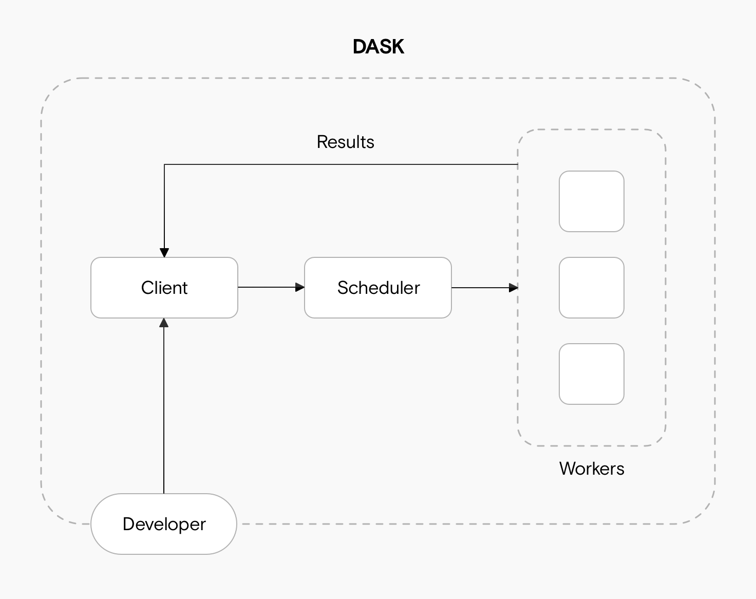
We can basically think of the Dask scheduler as our task orchestrator. To perform work, a scheduler must be assigned resources in the form of a Dask cluster. The Dask cluster has three main components for processing computations in parallel. These are the client, the scheduler, and the workers.

• The client is responsible for submitting tasks to be executed to the scheduler. It also enables you to monitor job progress and access the dashboard.

• The scheduler determines how client tasks will be distributed among the workers and coordinates the parallelized workload.

• The workers compute tasks and store and return computations results. Workers can be threads, processes, or separate machines in a cluster.

Setting up a Local Cluster

A LocalCluster runs all components on a single node and is useful for development and small-scale parallel workloads.

For this we need to set up a LocalCluster using dask.distributed and connect a client to it.

from dask.distributed import LocalCluster, Client

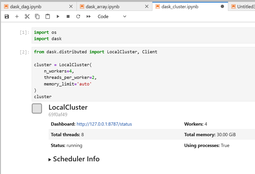
cluster = LocalCluster(
    n_workers=4,          
    threads_per_worker=2,
    memory_limit='auto'
)
cluster

• n_workers=4 creates four worker processes

• threads_per_worker=2 assigns two threads to each worker

• memory_limit='auto' lets Dask automatically manage memory allocation

Running the above code snippet provides the following output:

LocalCluster information:

Dashboard: http://127.0.0.1:8787/status
Total threads: 8
Status: running
Workers: 4
Using processes: True

If no arguments are provided, Dask will automatically configure workers based on available CPU cores and memory. In an Open OnDemand Jupyter session, this corresponds to the resources requested for that session.

Note

LocalCluster() can take additional (optional) arguments, allowing you to more precisely control its configuration. You can learn more about these arguments in the Dask online documentation.

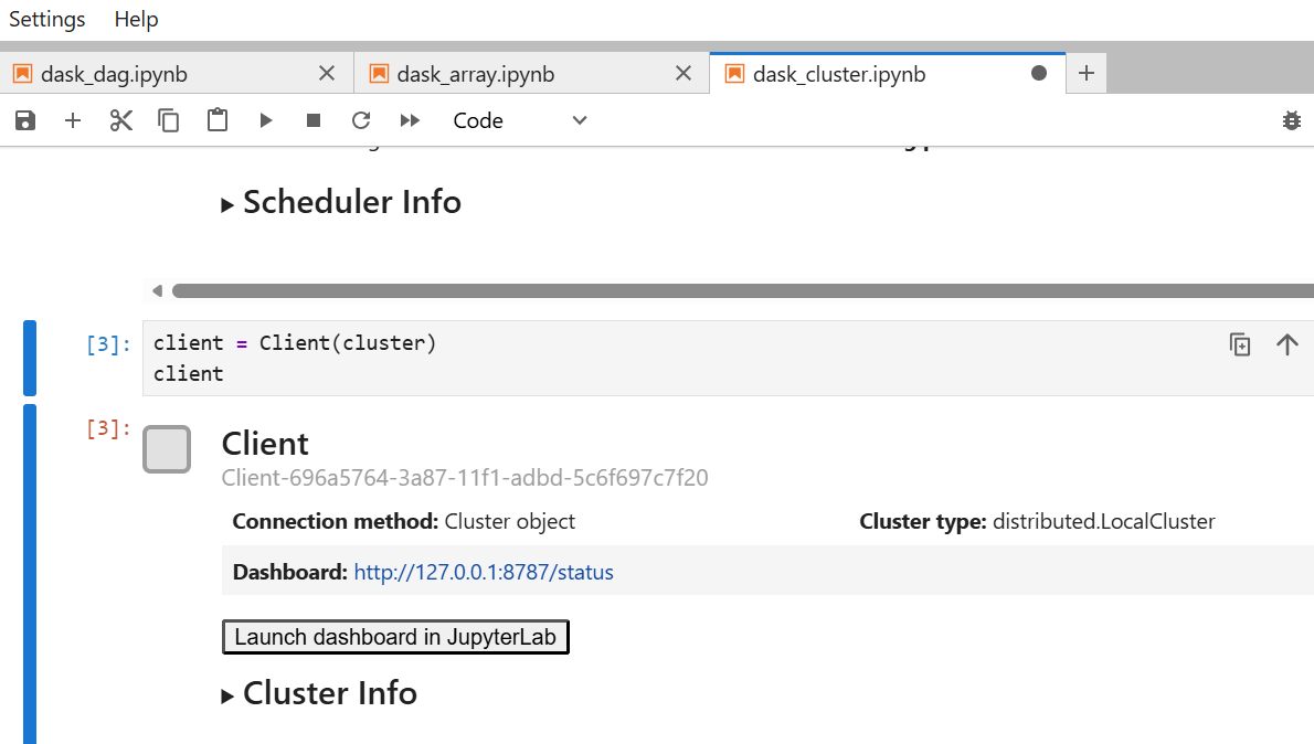
Once the cluster has been created, we will need to connect to through a client. To create a client, pass the cluster object to Client() function:

client = Client(cluster)
client

Through the client, you can run Dask commands and have the local cluster manager process your work. Once you have finished using the client, you will need to close the client in order to release its resources:

client.close()

If you have finished using the local cluster, you can similarly close it and release the cluster’s resources:

cluster.close()
# Or close both the client and cluster in one step:
client.shutdown()

Dask Dashboard

Dask comes with a really handy interface: the Dask Dashboard. It is a web interface that provides real-time insights into task execution, CPU and memory usage, and worker activity. You can retrieve the dashboard link using:

client

And in the dropdown menu on Cluster Info:

Dashboard http://127.0.0.1:8787/status
Total threads: 2
Status: running
Workers: 4
Using processes: True

The result of creating a Dask Client connected to a LocalCluster will look similar to the following:

Client ID: Client-696a5764-3a87-11f1-adbd-5c6f697c7f20
Connection method: Cluster object
Cluster type: distributed.LocalCluster
Dashboard: http://127.0.0.1:8787/status

You can also find your cluster dashboard link using :

cluster.dashboard_link

Warning

The provided link for the dashboard will not work in an Open OnDemand session as-is. The dashboard must be accessed through the Jupyter proxy.

For instructions on how to construct and access the correct URL, refer to: Connecting to the Dashboard

JupyterLab Plugin for Dask

Alternatively, you can access the Dask Dashboard using the JupyterLab plugin for Dask. This extension provides a graphical interface for launching clusters and viewing embedded dashboard panels directly within JupyterLab. Because JupyterLab extensions are tied to specific environments, you will need to create and use a dedicated Conda environment with the extension installed.

Step 1: Create a Conda Environment

#From a compute node
[johndoe@c3cpu-a5-u11-1 ~]$ module load anaconda
[johndoe@c3cpu-a5-u11-1 ~]$ conda create -n dask_lab_env python=3.10 -y
[johndoe@c3cpu-a5-u11-1 ~]$ conda activate dask_lab_env

Step 2: Install Required Packages

(dask_lab_env)[johndoe@c3cpu-a5-u11-1 ~]$ conda install -c conda-forge jupyterlab dask distributed

Then you can install the JupyterLab plugin for Dask

(dask_lab_env)[johndoe@c3cpu-a5-u11-1 ~]$ conda install -c conda-forge nodejs
(dask_lab_env)[johndoe@c3cpu-a5-u11-1 ~]$ conda install -c conda-forge dask-labextension

Step 3: Launch a Jupyter Session using your custom environment

Once your environment is set up, launch a Jupyter Session using the dask_lab_env environment that includes the extension.

Refer to the documentation here for detailed instructions on selecting and launching a jupyter session with custom Conda environment

Step 4: Use the Dask Extension

After launching JupyterLab, open the Dask tab from the left sidebar. The Dask icon appears alongside other JupyterLab tools such as the file browser and notebook panel.

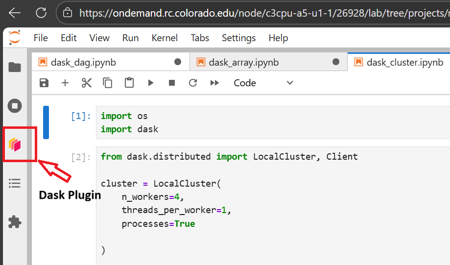
The following code demonstrates how a Dask cluster is created in the notebook environment:

import os
import dask
from dask.distributed import LocalCluster, Client

cluster = LocalCluster(
    n_workers=4,
    threads_per_worker=1,
    processes=True
)

Step 5: Connecting to the Dashboard

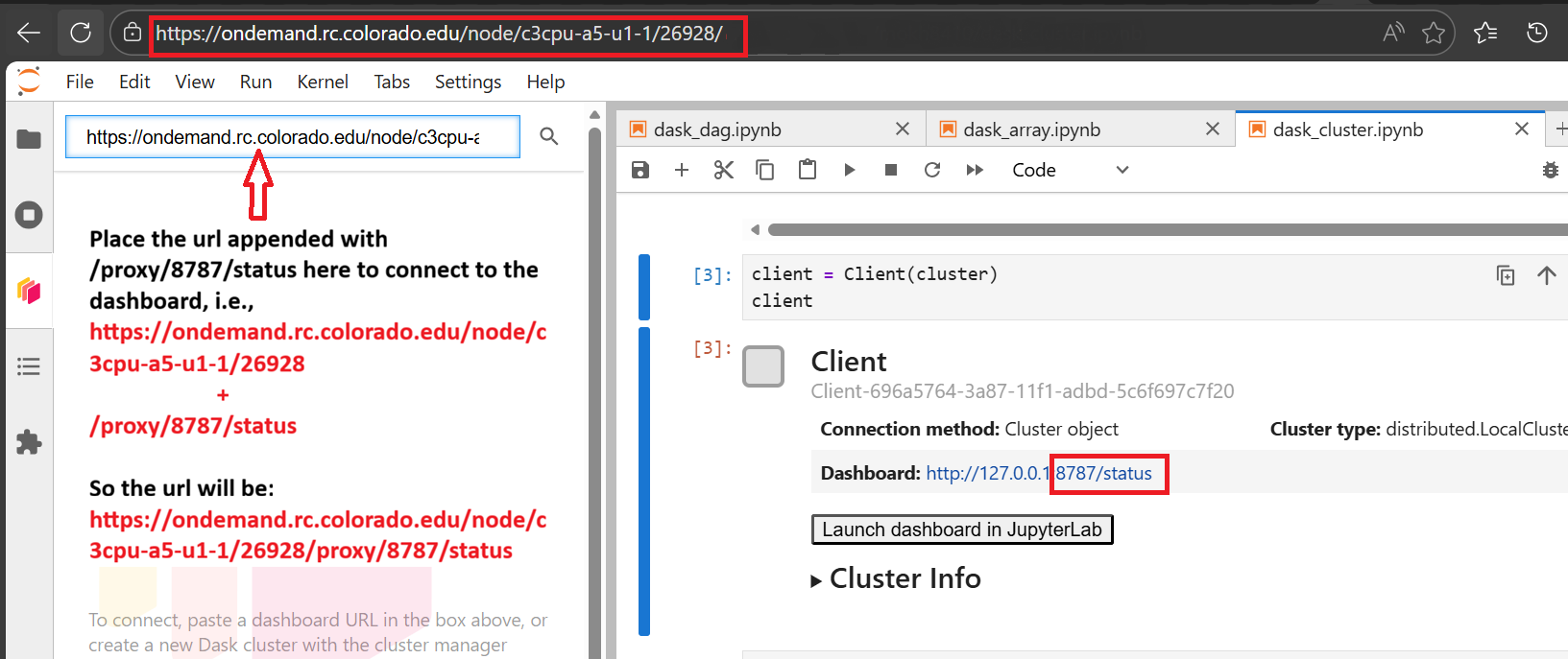
To connect the Dask extension to your running cluster, you must provide the dashboard URL.

In Open OnDemand, the dashboard cannot be accessed directly via 127.0.0.1. Instead, it must be routed through the Jupyter proxy.

Modifying the dashboard URL

Original dashboard URL:
http://127.0.0.1:8787/status

Open OnDemand session URL:
https://ondemand.rc.colorado.edu/node/<node-name>/<port>/

Accessible dashboard URL:
https://ondemand.rc.colorado.edu/node/<node-name>/<port>/proxy/8787/status

Step 6: Viewing the Connected Dashboard

Once the correct URL is entered, the Dask dashboard will connect and display live cluster metrics inside JupyterLab.

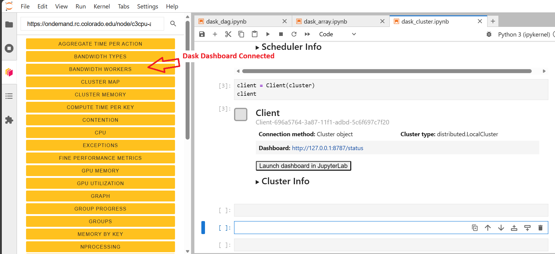
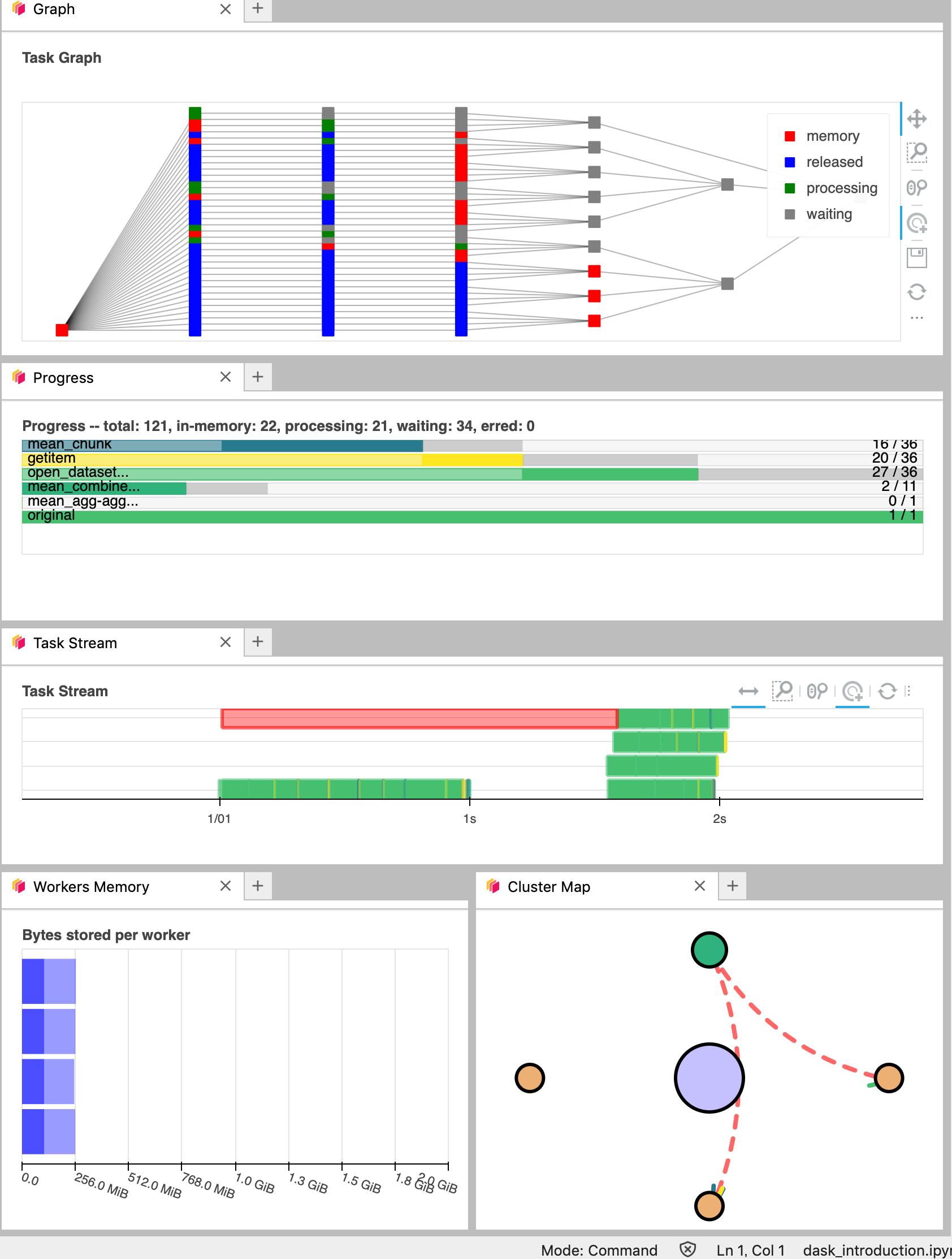
The dashboard includes multiple panels that display task execution, memory usage, worker activity, and performance metrics. You can click and drag the orange panels to rearrange the layout. This helps you track task progress visually, monitor resource usage and understand how work is distributed across workers.

Example: Estimating π with NumPy and Dask

In this example, we estimate the value of π using a Monte Carlo method. The initial implementation uses NumPy and runs serially.

This approach avoids explicit Python loops by leveraging vectorized NumPy operations. The computation generates random (x, y) points and determines how many fall inside the unit circle. As the number of sampled points increases, the estimate of π improves.

import numpy as np

def calculate_pi(size_in_bytes):
    
    """Calculate pi using a Monte Carlo method."""
    
    rand_array_shape = (int(size_in_bytes / 8 / 2), 2)
    
    # 2D random array with positions (x, y)
    xy = np.random.uniform(low=0.0, high=1.0, size=rand_array_shape)
    
    # check if position (x, y) is in unit circle
    xy_inside_circle = (xy ** 2).sum(axis=1) < 1

    # pi is the fraction of points in circle x 4
    pi = 4 * xy_inside_circle.sum() / xy_inside_circle.size

    print(f"\nfrom {xy.nbytes / 1e9} GB randomly chosen positions")
    print(f"   pi estimate: {pi}")
    print(f"   pi error: {abs(pi - np.pi)}\n")
    
    return pi

Serial Calculation (Baseline)

To evaluate Dask’s performance in calculating π, we will need an initial baseline to compare against. By running the code snippet and calling the calculate_pi function, we can determine how long it takes to run in serial using a single core.

Run the function:

%time calculate_pi(10000)

Output:

from 1e-05 GB randomly chosen positions
   pi estimate: 3.072
   pi error: 0.06959265358979305

CPU times: user 2.06 ms, sys: 1.44 ms, total: 3.5ms
Wall time: 2.78 ms

3.072

Parallelized Calculation with Dask

A key benefit of Dask is that it can parallelize computations without needing to modifying the original function (calculate_pi). By using dask.delayed, we construct a task graph that represents the computation.

from dask.distributed import Client
import dask

client = Client(n_workers=2, threads_per_worker=2, memory_limit="auto")

dask_calpi = dask.delayed(calculate_pi)(10000)

At this stage, the computation has not yet been executed. The delayed object defines the task, but execution is deferred.

To run the computation, use dask.compute:

%time dask.compute(dask_calpi)

Output:

from 1e-05 GB randomly chosen positions
   pi estimate: 3.0652
   pi error: 0.07639

CPU times: user 3.12 ms, sys: 1.51 ms, total: 4.63 ms
Wall time: 2.91 ms

3.0652

Visualizing the Task Graph

Dask provides tools to visualize how computations are structured. This can help identify parallelism and bottlenecks.

dask.visualize(dask_calpi)

Note

To use dask.visualize within JupyterLab, install the required dependency: conda install ipycytoscape.

The resulting graph shows a single task, indicating that no parallelism is being utilized.

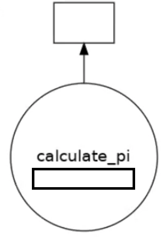
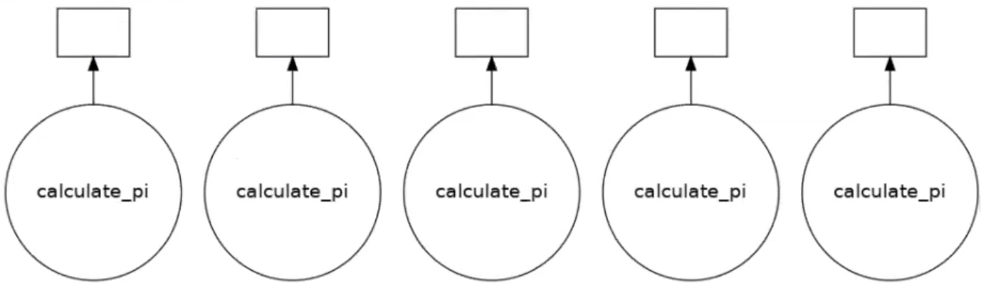
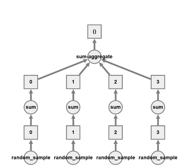
To take advantage of parallel execution, the workload must be split into multiple independent tasks. This can be done by invoking the function multiple times with different inputs.

results = []

for i in range(5):
    dask_calpi = dask.delayed(calculate_pi)(10000 * (i + 1))
    results.append(dask_calpi)

dask.visualize(results)

# Execute all tasks
# dask.compute(*results)

This produces a task graph with multiple independent tasks that can be executed concurrently across available workers.

Working with Data Structures

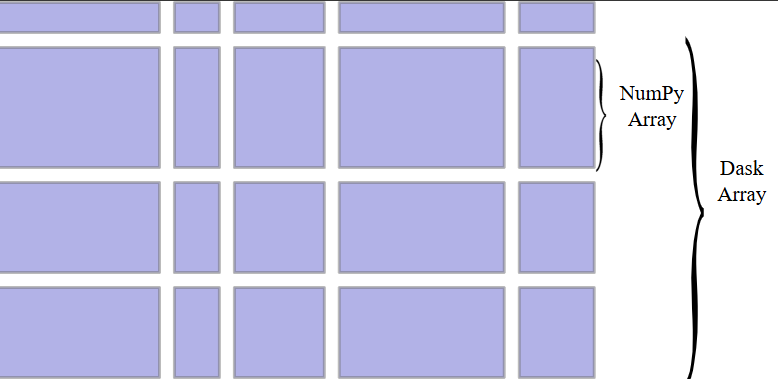
Dask Arrays

Dask Arrays are basically a parallelized version of NumPy arrays for processing larger-than-memory data sets. Each of these NumPy arrays within the dask.array is called a chunk. Choosing how these chunks are arranged within the dask.array and their size can significantly affect the performance of our code.

In the following example, we create a large random array using Dask and explicitly define how the array is divided into chunks.

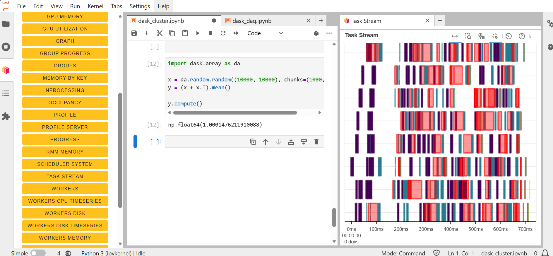
import dask.array as da
x = da.random.random((10000, 10000), chunks=(1000, 1000))

The Dask array has a total shape of 10,000 by 10,000, and it is divided into chunks of size 1,000 by 1,000. Each of these smaller chunks can be independently processed.

At this stage, no computation is performed. Dask only constructs a task graph that describes how the array should be computed.

Lazy Computation

We now define a computation on the array by combining it with its transpose and computing the mean.

y = (x + x.T).mean()

This operation creates a new expression that includes element-wise addition and a reduction step. However, no actual numerical computation is executed at this point. Instead, Dask continues to build the task graph that represents the computation. This lazy evaluation model allows Dask to optimize and schedule work before any data is loaded into memory.

To execute the computation and obtain a result, we explicitly call the compute method.

y.compute()

When this function is called, Dask evaluates the task graph by dividing the work into chunks, distributing the computation across available workers, executing tasks in parallel, and finally combining the intermediate results into a single output.

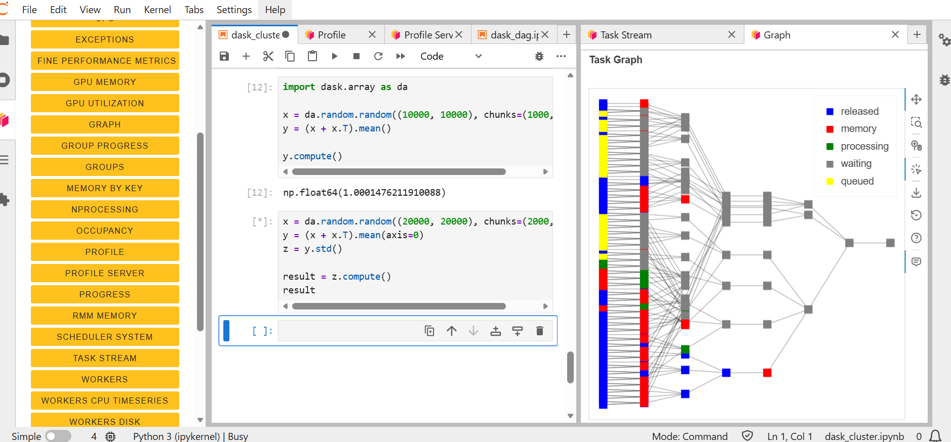
For a more complex workflow, involving multiple chained operations, use the following example:

x = da.random.random((20000, 20000), chunks=(2000, 2000))
y = (x + x.T).mean(axis=0)
z = y.std()

result = z.compute()
result

Here we first create a large 20,000 by 20,000 random array and divide it into chunks of 2,000 by 2,000. This results in a grid of independent blocks that can be processed in parallel. Then compute the sum of the array and its transpose, followed by a mean across axis 0. This operation reduces the dimensionality of the dataset but still remains in a lazy state. We perform a second transofrmation, computing the standard deviation of the intermediate result. Finally, we call compute on the result.

Blocked Algorithms

Dask Arrays are implemented using blocked algorithms. These algorithms break up a computation on a large array into many computations on smaller pieces of the array. This minimizes the memory load (amount of RAM) of computations and allows for working with larger-than-memory datasets in parallel.

Let’s see what this means in an example:

x = da.random.random(20, chunks=5)
result = x.sum()

result.compute()
# result.visualize() #uncomment to visualise it

This will generate a random array, and it will automatically create the tasks, and from there the sums will be parallelised. This is similar to what you would see in MPI, but much easier to implement.

Dask Dataframes

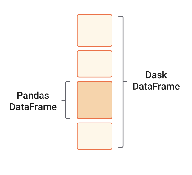
When we analyze tabular data, we usually start our analysis by loading it into memory as a Pandas DataFrame. But what if this data does not fit in memory? In such cases, Dask’s scalable alternative to a Pandas DataFrame is the dask.dataframe. A dask.dataframe comprises many pd.DataFrames, each containing a subset of rows of the original dataset. We call each of these pandas pieces a partition of the dask.dataframe.

In short: Dask DataFrames extend pandas for parallel and out-of-core data processing.

A simple example for this would be:

1. Creating a Dask DataFrame

import dask.dataframe as dd
df = dd.read_csv("data/file.csv")
df

This creates a lazy DataFrame composed of many partitions.

2. Basic Data Operations:

#filter operation
filtered = df[df["column"] > 10]

# Groupby operation
grouped = filtered.groupby("category").mean()
grouped

Keep in mind that nothing is computed yet.

3. Trigger Computation:

result = grouped.compute()

Now Dask processes each partition in parallel and combines results.

Tip

Before calling compute on an object, open the Dask dashboard to see how the parallel computation is happening.